Introduction to Significance Testing

Flukes versus meaningful results

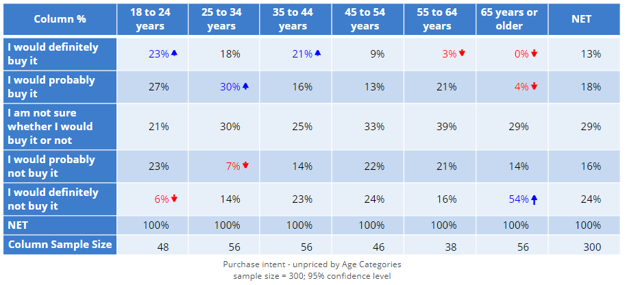
The crosstab below shows how likely people said they would be to purchase an iLock, by age category. In the total sample of 300 people (the NET column), 13% said they would definitely buy it. Looking at the first row of the table, we can see that younger people are more likely to say they will definitely buy it, and older people are less likely to buy it. Intuitively this makes sense. But, the sample size is only 300 and the sample size in each age band is only about 50. Maybe the result is just a fluke, and if we were to repeat this study again, with a different 300 people we would get a different result, and find that older people are more likely to say they will buy the product.

So, the problem to be solved is to work out if an interesting result is likely a fluke, or, is likely to reflect some truth that has been uncovered by the survey. Fortunately, some clever math has been invented that answers such questions, and this math is variously known as stat testing, significance testing, sig testing, and statistical inference, as well as some other names.

Exception tests

With tables showing column percentages, like the one above, we are interested in comparing the numbers across rows. If all the numbers in each row were the same, then the data suggests that purchase intent is unrelated to age.

Exception tests on tables with column percentages check to see if any of the results in the table are exceptions to the "rule" that there are no differences in a row. 

No exceptions

Look at the row which shows I am not sure whether I would buy it or not. None of the results in this row have colors or arrows next to them. This doesn't mean that all the results in the row are the same. They clearly are not, varying from 21% to 39%. What it means is that the observed variation is not exceptional. Or, to put it a different way, the observed variation in this row is in line with what we would expect for a study like this.

Exceptionally high results

The table is reproduced below so you don't have to scroll. In the first row, you can see that there are two cells that are blue with arrows pointing upwards. This tells us that these two results are exceptionally high, where "exceptional" in this context means they are exceptions to the rule that there is no difference in the column percentages.

More precisely, we can say that the 23% result for 18 to 24 years is significantly higher than the result for all the other age groups (i.e., people aged 25 or more).  Similarly, the 21% result for the 35 to 44 years category is also significantly high.  

Significantly low results

We can also see that the results of 3% and 0% for the 55 to 64  and 65+ categories are exceptionally low. This is indicated by the red and the downward arrows.

P-values

The chart below shows the column percentages from the first row of the table. The two age categories marked on the table as being significantly high are the ones with the highest values. The age categories with the lowest results are marked as being significantly low. What does this mean about the in-between ones? For example, does this imply that the proportion of the 25 to 34 years category that said they would definitely buy is no higher than the rest of the age groups? No, it doesn't. Just looking at the chart below and a bit of common sense makes it seem likely that the 25 to 34 year age group are more likely to say they definitely will buy the product. This begs the question: why aren't they marked as being significant?

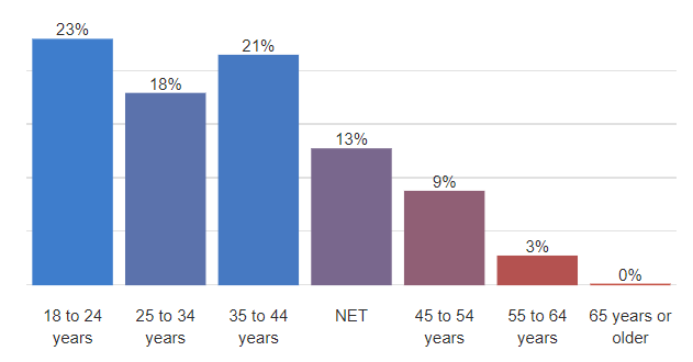
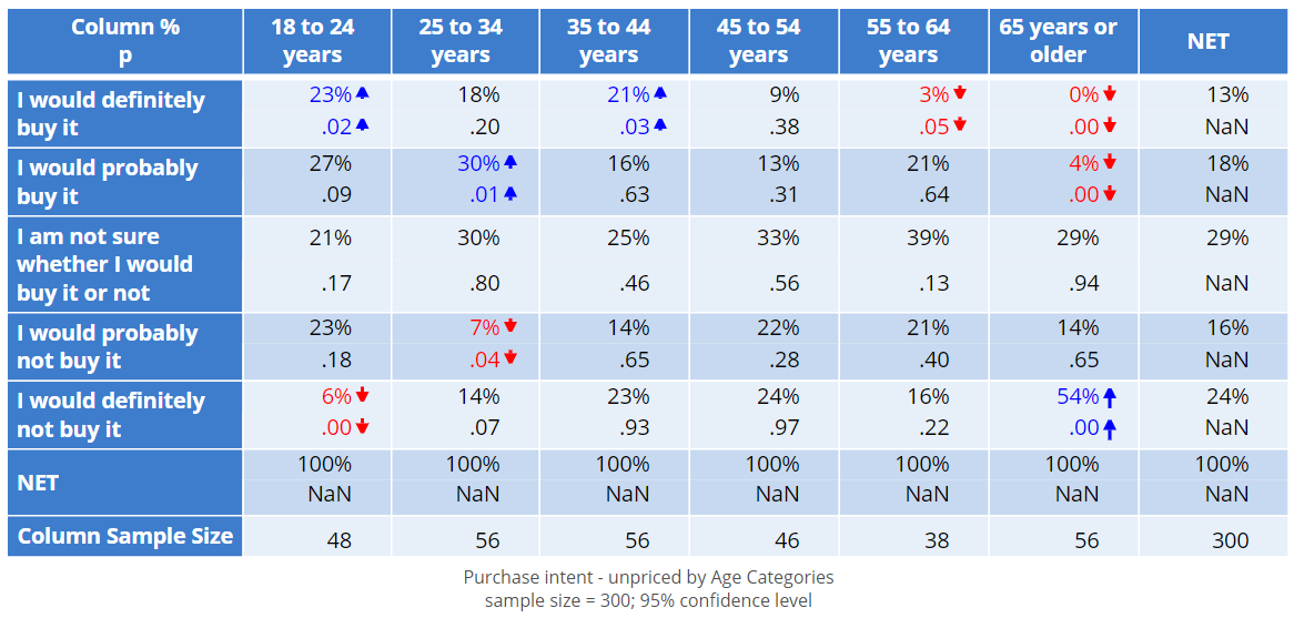
Any result must fall on a continuum from being entirely unexceptional (i.e., not different), through to being highly exceptionally (very different). The p-value is the most widely used statistic for quantifying how exceptional a result is, where the p refers to a probability (the exact definition of the probability is outside the scope of this introductory article).

By convention, when the p-value is less than or equal to 0.05, the result is regarded as being sufficiently exceptional and is tagged as being "significant". So, the 25 to 34 years category has a percentage that is clearly higher than the NET (18% versus 13%). But, its magnitude of 0.05 is not big enough for us to mark it as being significant.

Confidence levels

Sometimes people refer to confidence levels rather than p-values. These are equivalent ideas. A p-value of 0.05 is the same thing as the result is significant at the 95% level of confidence. That is:
100 - 100p = Confidence.

The need for common sense

The cutoff p-value of 0.05 is arbitrary. Is it a smarter cutoff to use than, say, .1 (90% confidence), or 0.02 (98% confidence)? Maybe. Maybe not. The only reason 0.05 is widely used is it was proposed by one of the great minds of the 20th century, Sir Ronald Fisher, and if we are going to have an arbitrary number, it may as well be his.

However, it is very, very important to appreciate that the cutoff is often wrong. A result will be marked as being significant when it is in fact a fluke. And, results will be shown as being not significant when in fact they really reveal something important insight into the world.

For this reason, a good practice is to use common sense when reviewing the results, looking at the overall trends in the data, and, where possible, triangulating results with other data from other studies. For example, if you just summarized the results of the significance tests literally you would arrive at the result on the left. However, the interpretation on the right is a more sensible one.

Pairwise column comparisons

So far we have been looking at exception tests. Another type of widely used approach to significance testing is to use pairwise column comparisons. These compare each pair of columns, using letters to denote the results of the significance tests.

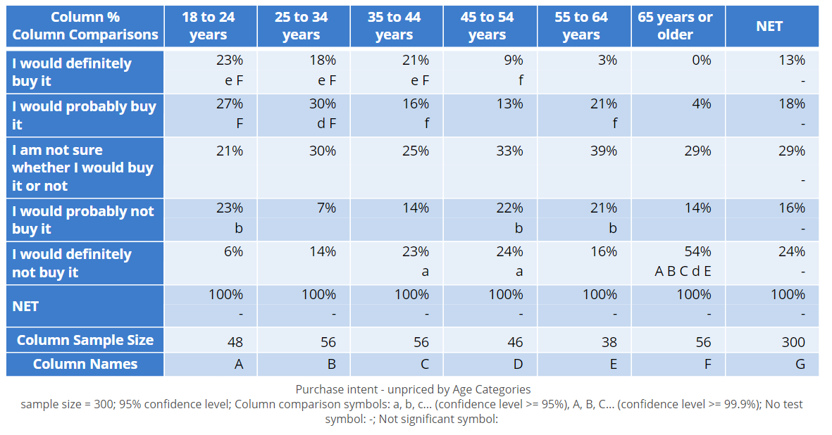
In the table below, each of the columns has been given a label (shown at the bottom). The 18 to 24 years column is A, the next is B, etc.  These letters are read as follows:

• The letter e for the 18 to 24 years group in the first row is telling us that the 23% for this group is significantly higher than the 3% for column E (55 to 64 years).
• The letters are only shown for the higher of the pair of columns. So, there is nothing in column E nor F indicating it is lower than A.
• The letter F for the 18 to 24 years group is telling us that the 23% for this group is significantly higher than the 0% for column F (65 years or older).
• The reason that the e is lowercase but the F is uppercase, is that the software used to create the table has used two different cutoff values. Lowercase letters denote p-values of less than 0.05 (95% level of confidence). Uppercase denotes p-values of less than 0.001 (99.9% level of confidence).
• The 25 to 35 years and 35 to 44 years are also significantly higher than 55 to 64 years and 65 years or older.
• 45 to 54 years is significantly higher than 65 years or older.

As with exception tests, a good practice is to apply common sense and synthesize the results:

Significance levels and exception tests

A nice feature of the pairwise column comparisons is that it showed two levels of significance, by the lower and uppercase letters. This has also been done in the exception tests, where longer arrows denote smaller p-values. This allows us to quickly see in the table below that the interest in the product is really very low among the 65 years or older age category. 

Which significance test to use when

In this article, we have looked at exception tests and pairwise column comparisons. Which of these should you use and when? 

The exception tests are easier to read, faster to read, and more powerful (which is statistical jargon for better in this context). However, the pairwise column comparisons are:

• More traditional, and many people still expect them.
• More appropriate if you are only interested in a subset of possible comparisons between the columns.